regression cycle
Two different variables were used for prediction in the model: fantasy_value_per_game(fvpg), and draft_capital. The process predictive_age(p_age) 21-44, dependent_age(d_age) 21-45, and games_played(gp) 0-80, each time performing an , . Data used was from NFL seasons 2005-2020.
Dependent_value is determined each iteration by adding fantasy_value(fv) from weeks 1-17. Data had to be filtered to exclude players who haven't played in those seasons, by the following conditions:
- any player who's age in 2020 was less than d_age
- any player who's age in 2005 was greater than or equal to p_age
- any player who's rookie age was less than p_age
- any player who had played in less games at the given p_age than the lower bound of gp
For an example, consider Odell Beckham Jr. who turned 28 in 2020, and Terrell Owens who turned 32 in 2005. OBJ would need to be be excluded from any regression in the cycle where d_age is greater than 28 because he hadn't even played yet. T.O.'s instance is not included any time p_age is less than 32 since said season occured before 2005.
The fv metric happens to also act as the , meaning this portion of the model is an .
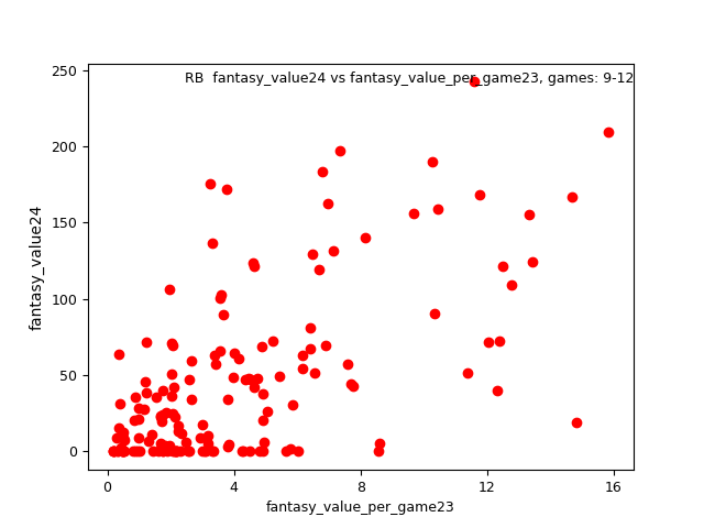
The function takes fvpg at one age to predict fv at a later age.
The example below visualizes RB age 23 fvpg correlation with age 24 fv:
The lower and upper bounds of games_played cycled the following values: 1-1, 2-2, 3-3, 4-4, 5-5, 6-6, 7-8, 9-11, 12-16, 17-32, 33-48, 49-64, 65-80. The aim is to articulate a relationship between gp and better prediction. It stands to reason that one who has been in 30 games offers more confidence than a player who's been in just 1.
With every iteration, predictive_value(pv) was calculated by summing fv from the most recent game going backwards, counting each game until the upper bound of gp was met; predictive_games_played(pgp) is equal to the count of games. The summation continued beyond the p_age when necessary, but only back 4 seasons. Any player who appeard in fewer games than the lower bound of gp was not included. Since the interest here is how past performance translates in the future, any player who had predictive_value of 0 was also filtered into a seperate data set.
Each regression returns the parameters of a , slope and y-intercept. The computer uses the process of to estimate these parameters. But, in this case the value of the y-intercept can be determined exactly. Consider in a linear function the equals y when x = 0. Described in the last paragraph, players with pv of zero were removed, seperated into another data set; this filtered out sample can be said to represent dependent_value(dv) when pv = 0. A new variable intercept is defined to equal this sample's mean dv.
The slope parameter still needs to be estimated, for which is invoked. Fortunately, this is an option of the python library. Another transformation is needed wherein a new variable dependent_value_adjusted(dv_adj) is defined according to the following algebra:
dv = slope * pvpg + intercept
dv - intercept = slope * pvpg
dv_adj = dv - intercept
dv_adj = slope * pvpg
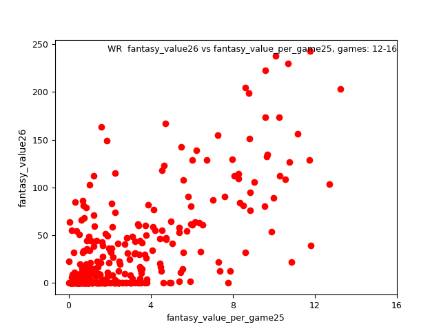
To make a , players who had no fantasy_value in the predictive_age were removed, their average fantasy_value in the dependent_age was subtracted from the dependent_value in the iteration's training data set. This adjusted fantasy_value in the dependent_age was used as the dependent variable in the regression analysis. This process only works by forcing the regression thru the origin.
Results are visualized for your information, below shows a scatter plot of the WR position, p_age 25, d_age 26, gp 12-16:
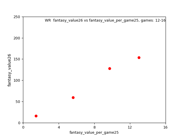
Again aggregating values into bins, making the trend more apparent:
The following links show all the visualizations, scatter plots, and binned scatter plots;
and including the trend lines, binned scatter plots, regression summaries.
Some of them don't always look perfect, but remember the purpose purpose behind all the iterations seeks a holistic approach.
residuals
, also known as error, equal real values minus predicted values. These are used to judge a regression's goodness of fit. For example, standard deviation is equal to the square-root of the average squared residual, which is used for prediction intervals and determining R2. It's also necessary to reveiw residuals in checking the of simple linear regression:
- Trend is linear
- No heteroscedasticity in residuals
- Residuals have a
- of residuals
Histograms seem to follow a normal distribution.
Here's one for receiver:

Albeit they show some , resulting from the fact fv, as its defined, cannot fall below zero.
Predictions resembles a little bit of a by always predicting less fv in the d_age than players have in the p_age.
On average, this is the way it works out in real life, so , but can explain the residual distribution.
The residuals vs predictions scatter plots are a convoluted mess, easier to comprehend by looking at each iteration individually. You can cycle thru these residual diagrams on your own if you wish. These are reviewed to check the assumptions listed above. doesn't appear to be an issue.
But independence is a bit more , basically meaning the residuals do not relate to any other factor.
The process already is by cycling measures of gp, p_age, and d_age.
But time was not considered.
Data was gathered from 2005-2020, whatever trend exists from the NFL evolving during this period is not captured by the model;
so it's necessary to review residuals vs predictive_year, shown here.
This one is of TE, all iterations:
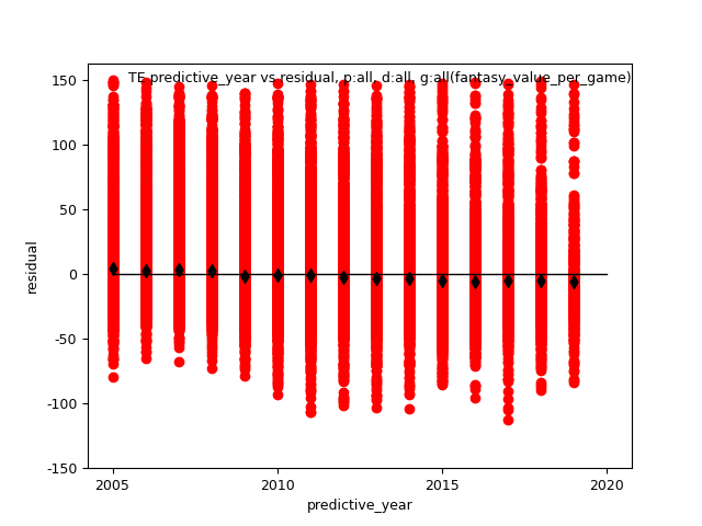
Black diamonds represent the average residual of each predictive_year, which show a very slight trend negative trend.
The same tendency is observed of RB, WR, an indication fv has increased marginally with time.
In my opinion, not enough to cause an issue, since the change is minimal.