draft capital
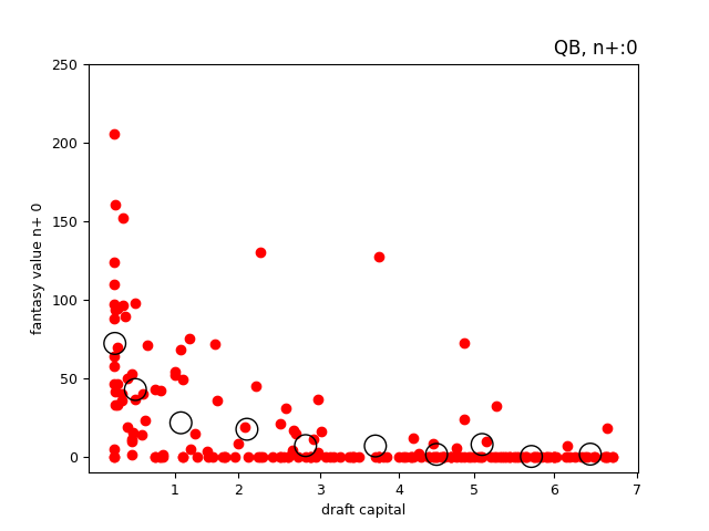
The cycle of regressions for the draft capital variable was done differently than fantasy_value_per_game. We originally hypothesized that a player's draft age was a , but in the end this was found to be a case of . The process was instead simplified to loop only thru the n+ variable. In other words, the only other factor considered in addition to draft_capital, was NFL experience.
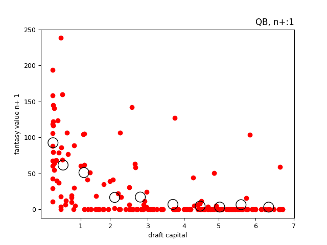
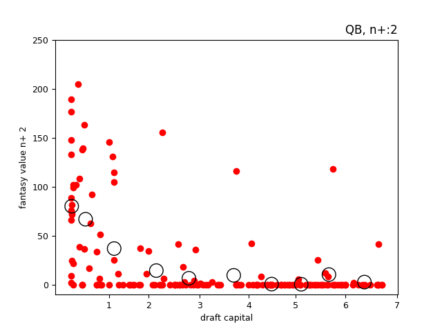
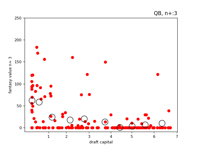
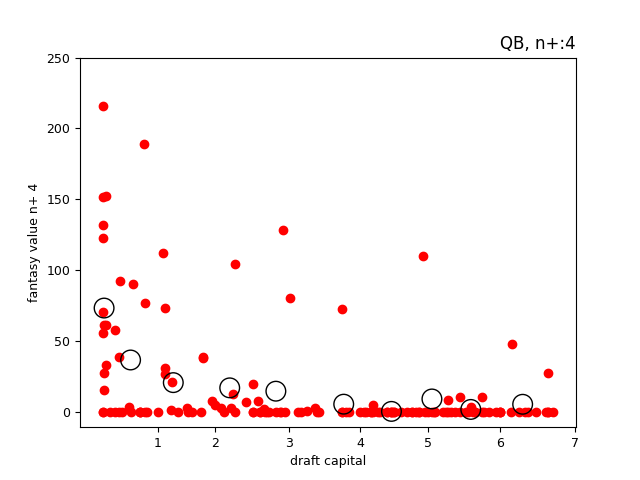
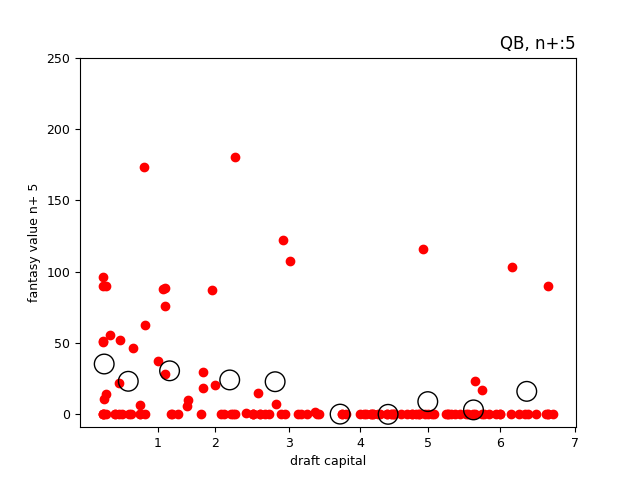
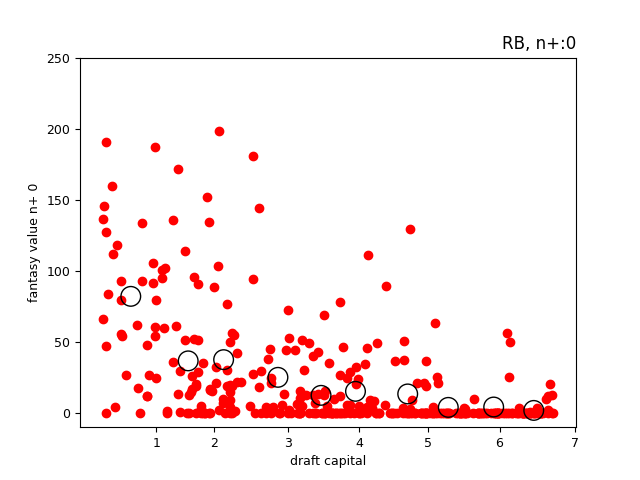
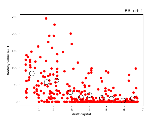
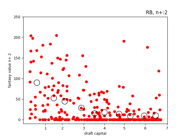
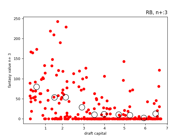
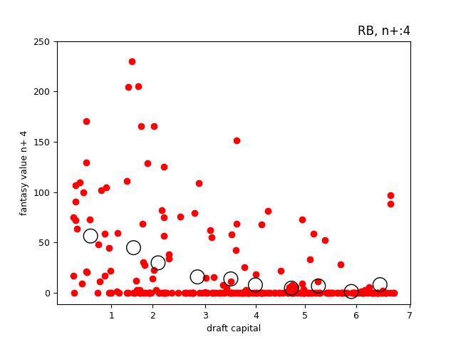
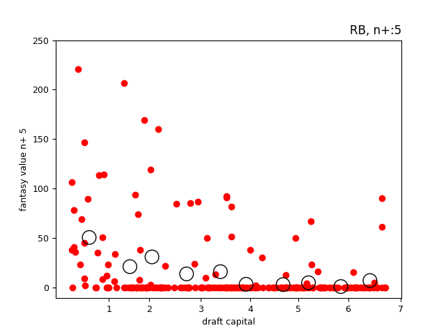
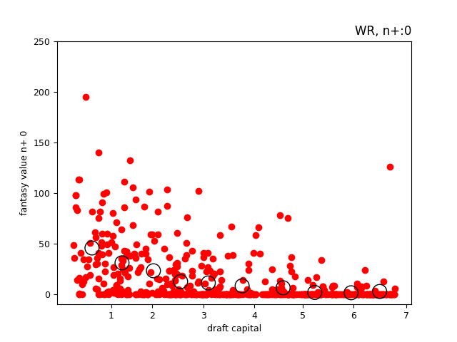
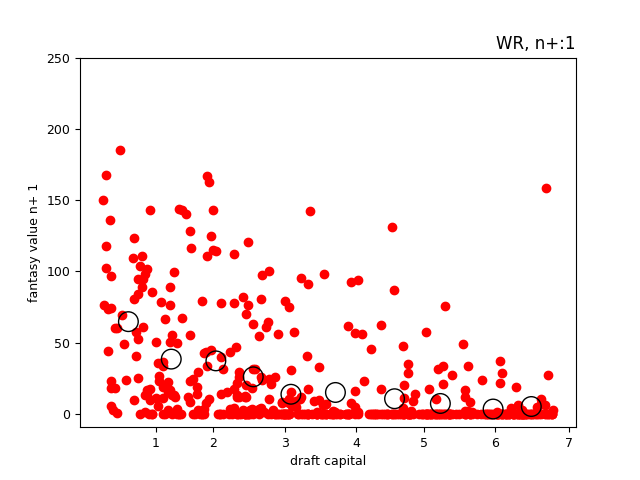
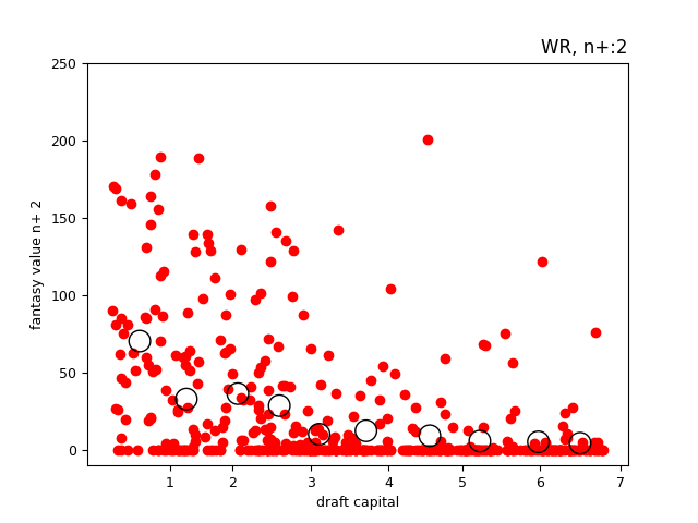
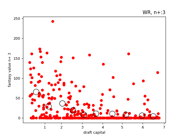
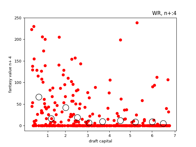
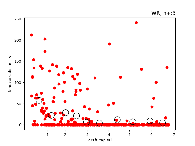
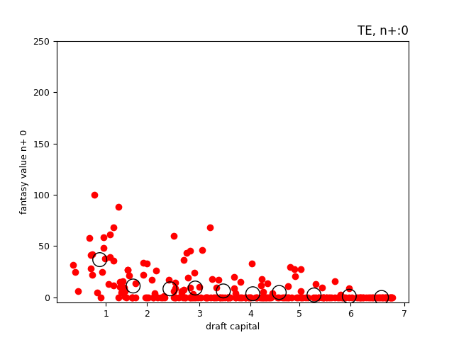
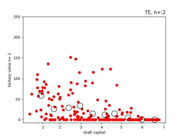
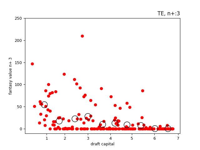
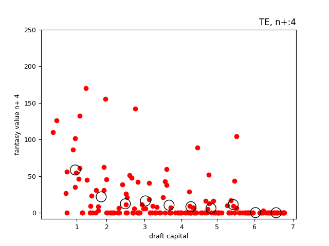
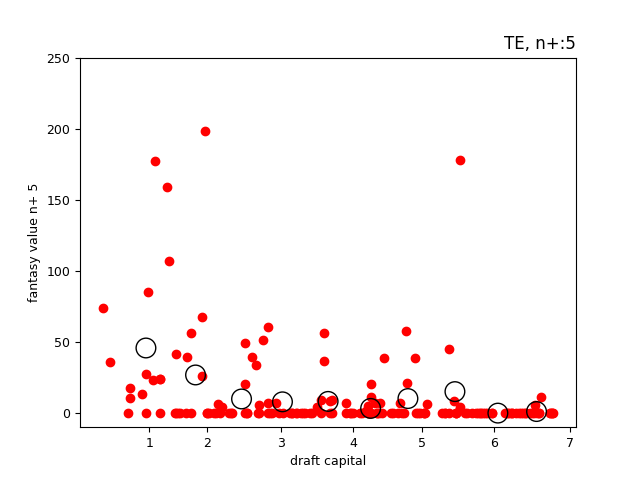
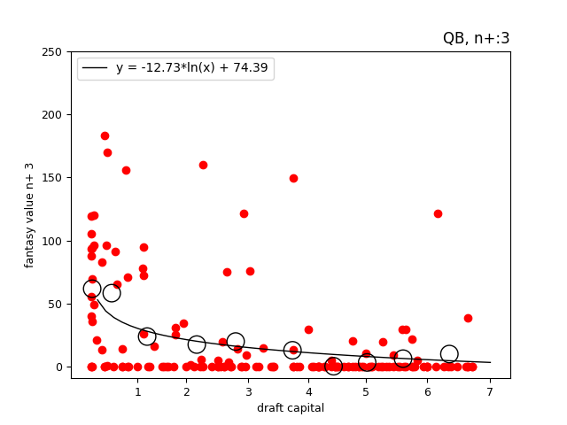
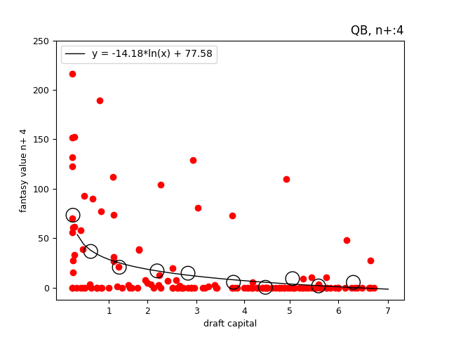
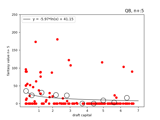
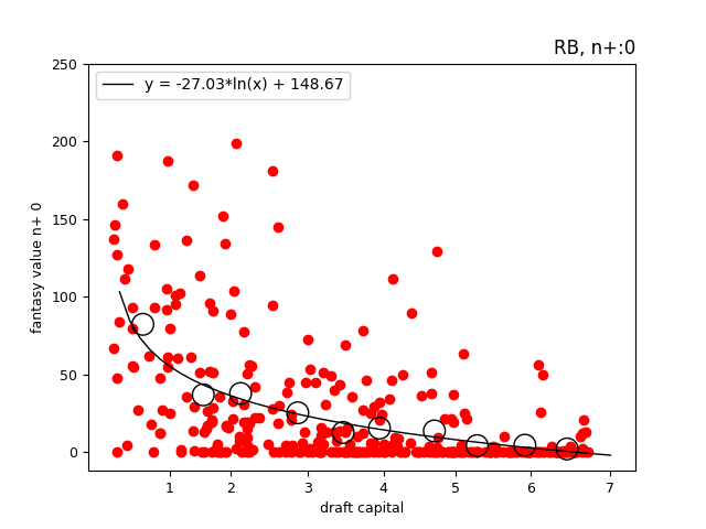
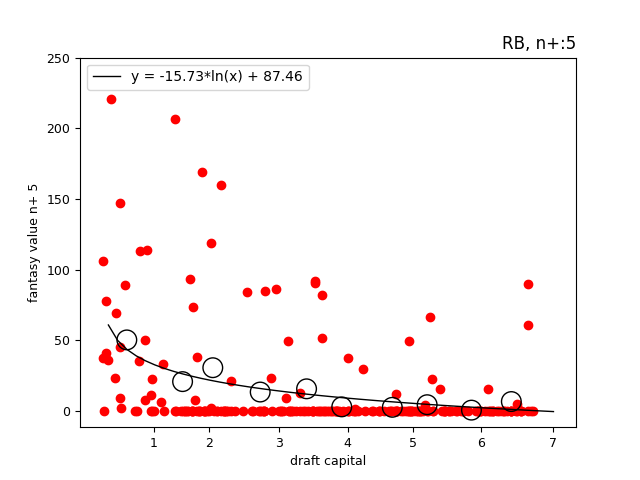
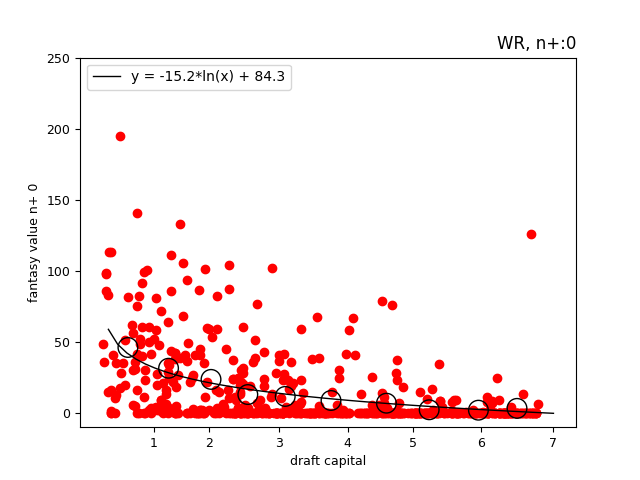
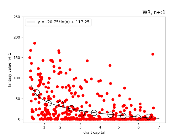
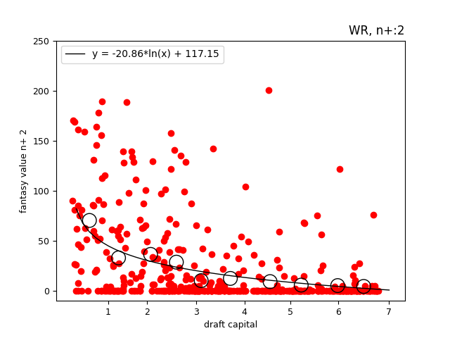
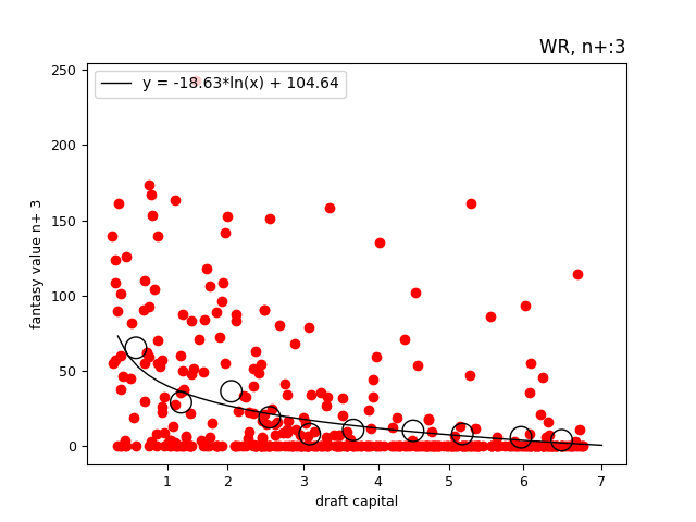
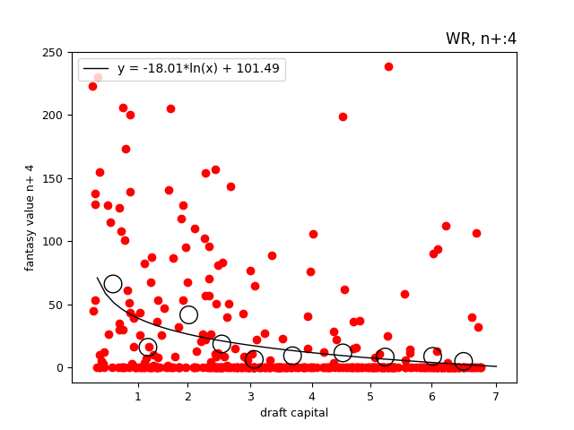
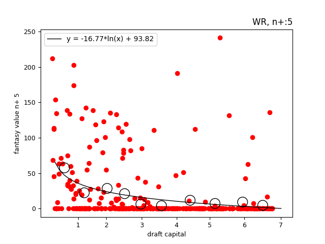
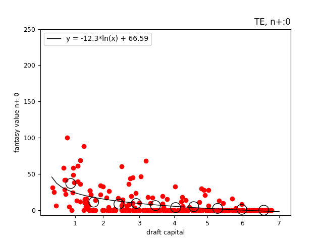
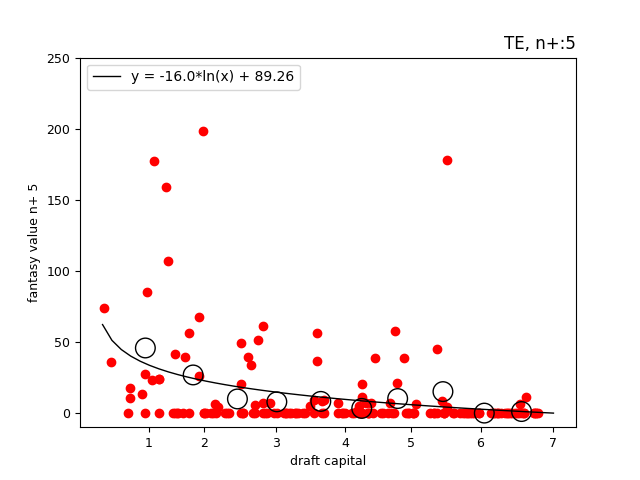
One complication came up, that draft_capital didn't fit with a straight line. Upon scrolling thru the following images, you can see what I mean. The larger circles in the following scatter plots reperesent bin averages of each 10th percentile; these percentiles were added to make the trends easier to see.
QB:
RB:
WR:
TE:

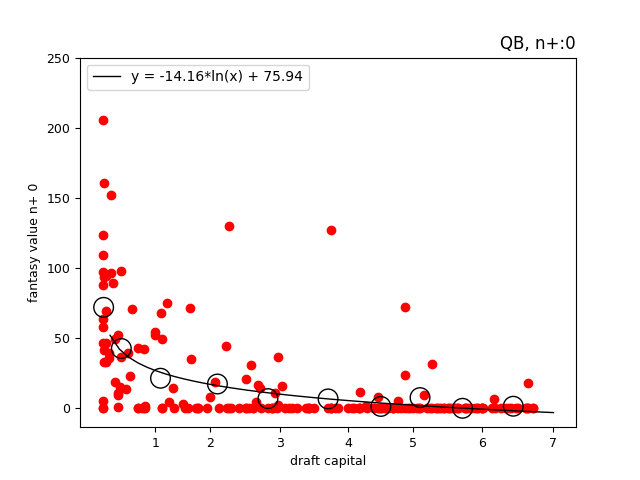
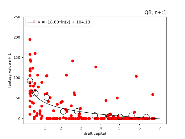
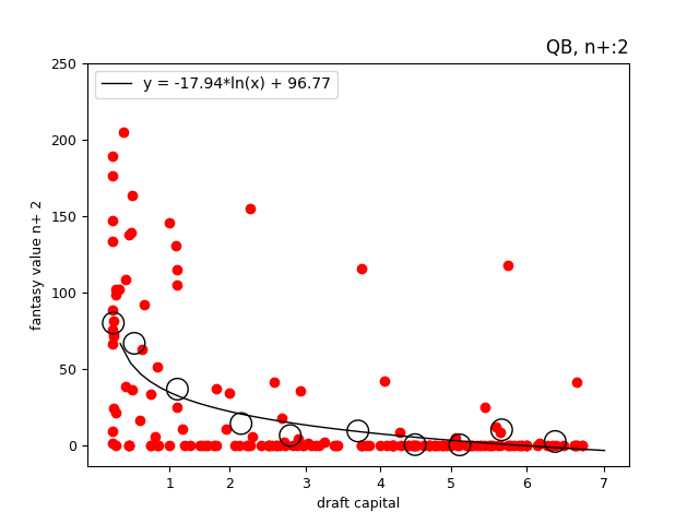
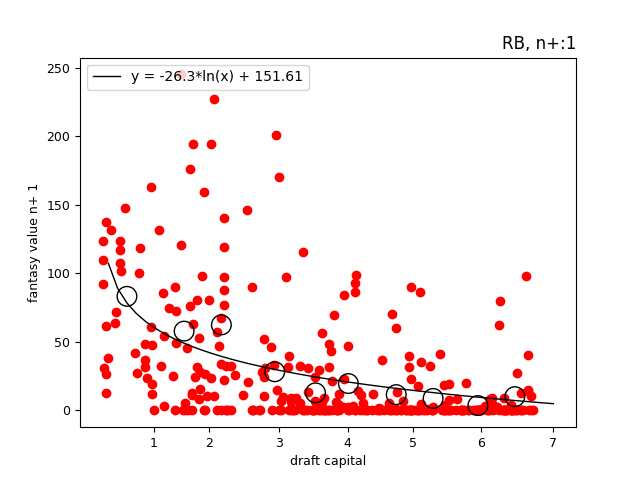
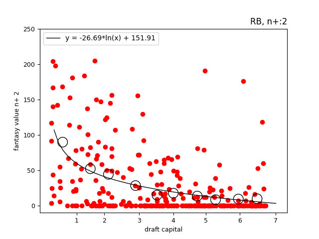
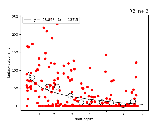
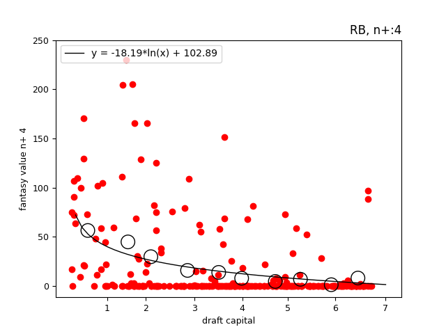
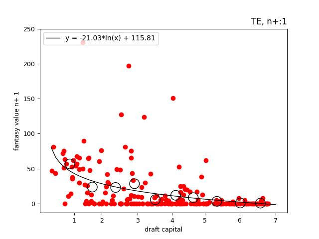
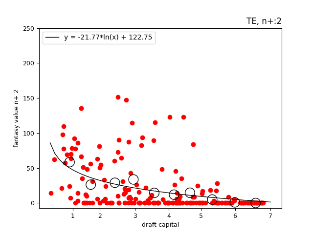
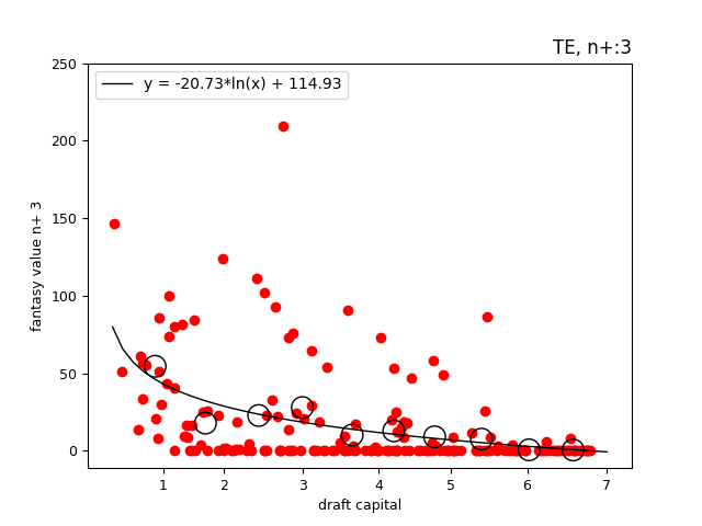
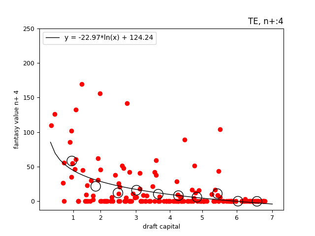
The next group of images shows the same thing except with a trend of best fit included. In the top right corner you'll find each trend's formula from the completed regression.
QB:
RB:
WR:
TE:
The graphs only show n+ 0-5, but the regressions were completed up to 14, just in case was needed. The following table displays all the regression parameters for each position. You can see
| pos | n+ | y intercept | slope | R2 |
|---|---|---|---|---|
| QB | 0 | 75.9 | -14.2 | 0.403 |
| QB | 1 | 104.1 | -18.9 | 0.381 |
| QB | 2 | 96.8 | -17.9 | 0.366 |
| QB | 3 | 74.4 | -12.7 | 0.223 |
| QB | 4 | 77.6 | -14.2 | 0.282 |
| QB | 5 | 41.1 | -6.0 | 0.062 |
| QB | 6 | 67.0 | -12.1 | 0.193 |
| QB | 7 | 44.8 | -8.0 | 0.133 |
| QB | 8 | 47.8 | -8.3 | 0.116 |
| QB | 9 | 43.6 | -8.2 | 0.179 |
| QB | 10 | 46.8 | -8.8 | 0.162 |
| QB | 11 | 51.5 | -10.0 | 0.198 |
| QB | 12 | 53.7 | -109 | 0.305 |
| QB | 13 | 15.8 | -2.1 | 0.011 |
| QB | 14 | 6.5 | -0.2 | 0.001 |
| - | - | - | - | - |
| RB | 0 | 148.7 | -27.0 | 0.361 |
| RB | 1 | 151.6 | -26.3 | 0.238 |
| RB | 2 | 151.9 | -26.7 | 0.246 |
| RB | 3 | 137.4 | -23.8 | 0.199 |
| RB | 4 | 102.9 | -18.2 | 0.171 |
| RB | 5 | 87.5 | -15.7 | 0.141 |
| RB | 6 | 59.4 | -10.3 | 0.090 |
| RB | 7 | 52.6 | -9.5 | 0.108 |
| RB | 8 | 29.5 | -5.4 | 0.063 |
| RB | 9 | 12.7 | -2.2 | 0.023 |
| RB | 10 | 12.9 | -2.3 | 0.043 |
| RB | 11 | 11.9 | -2.2 | 0.037 |
| RB | 12 | 6.3 | -1.2 | 0.27 |
| RB | 13 | 5.1 | -0.9 | 0.046 |
| RB | 14 | 0.6 | 0.0 | 0.000 |
| - | - | - | - | - |
| WR | 0 | 84.3 | -15.2 | 0.250 |
| WR | 1 | 117.2 | -20.8 | 0.238 |
| WR | 2 | 117.2 | -20.9 | 0.216 |
| WR | 3 | 104.6 | -18.6 | 0.195 |
| WR | 4 | 101.5 | -18.0 | 0.143 |
| WR | 5 | 93.8 | -16.8 | 0.140 |
| WR | 6 | 82.3 | -15.0 | 0.125 |
| WR | 7 | 58.2 | -10.5 | 0.084 |
| WR | 8 | 44.4 | -8.0 | 0.067 |
| WR | 9 | 20.7 | -3.5 | 0.024 |
| WR | 10 | 7.1 | -0.9 | 0.003 |
| WR | 11 | 1.7 | -0.3 | 0.007 |
| WR | 12 | 1.7 | -0.3 | 0.045 |
| WR | 13 | 0 | 0 | 0.000 |
| WR | 14 | 0 | 0 | 0.000 |
| - | - | - | - | - |
| TE | 0 | 66.6 | -12.3 | 0.277 |
| TE | 1 | 115.8 | -21.0 | 0.219 |
| TE | 2 | 122.8 | -21.8 | 0.201 |
| TE | 3 | 114.9 | -20.7 | 0.210 |
| TE | 4 | 124.2 | -23.0 | 0.251 |
| TE | 5 | 89.3 | -16.0 | 0.112 |
| TE | 6 | 85.2 | -15.6 | 0.166 |
| TE | 7 | 98.9 | -18.3 | 0.140 |
| TE | 8 | 47.3 | -8.5 | 0.085 |
| TE | 9 | 37.1 | -6.7 | 0.047 |
| TE | 10 | 36.1 | -6.6 | 0.064 |
| TE | 11 | 35.5 | -6.7 | 0.111 |
| TE | 12 | 24.3 | -4.8 | 0.197 |
| TE | 13 | 7.5 | -1.4 | 0.086 |
| TE | 14 | 0 | 0 | 0.000 |
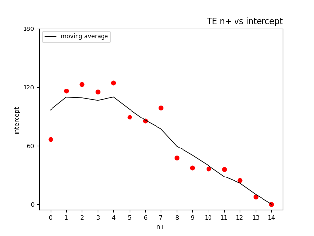
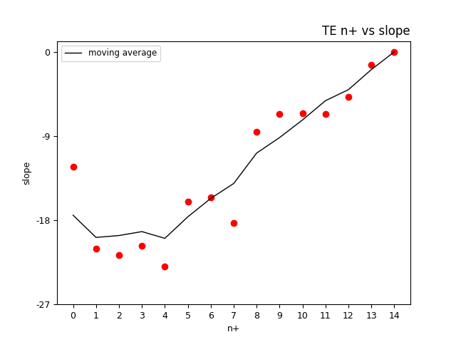
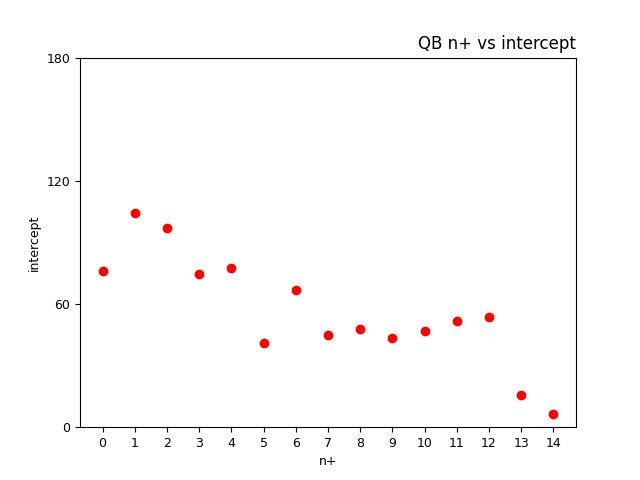
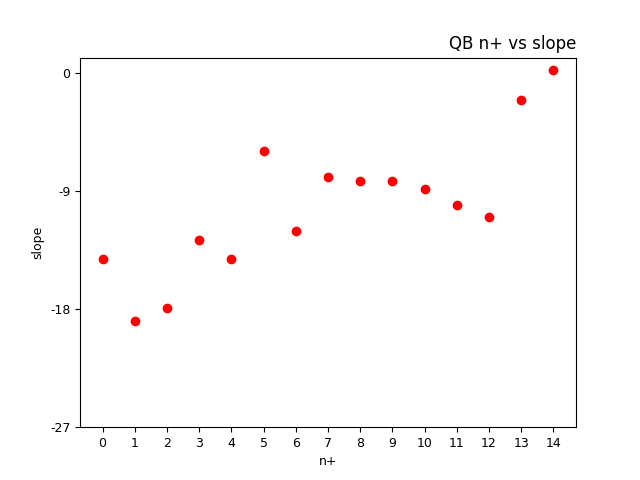
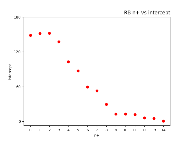
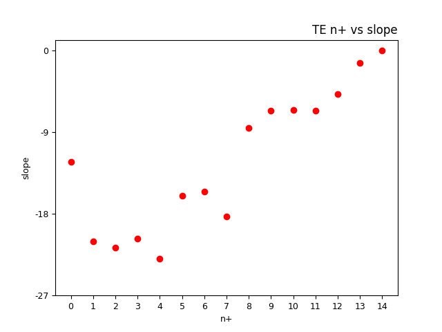
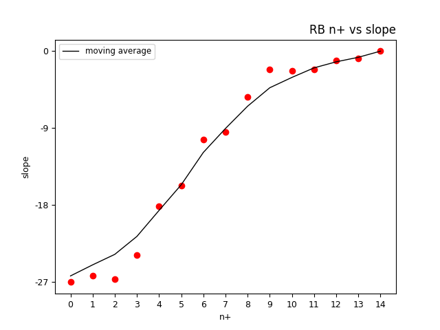
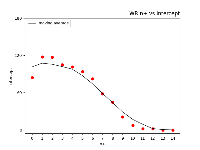
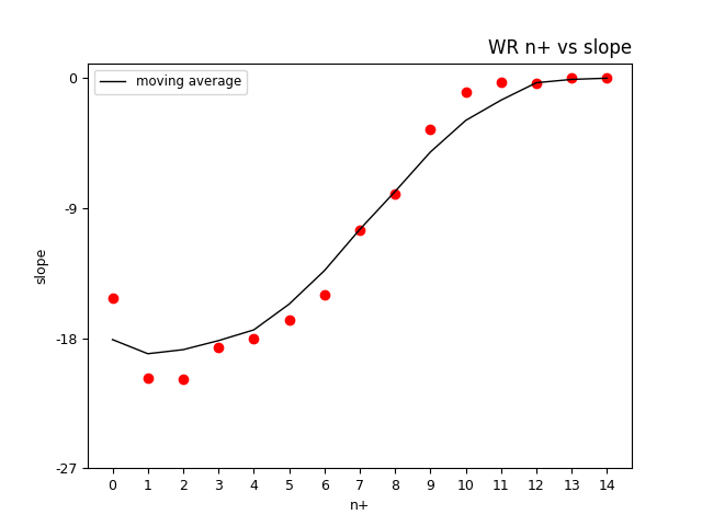
The next group of images below graphically displays the parameters of slope and y-intercept from the previous table.
QB:
RB:
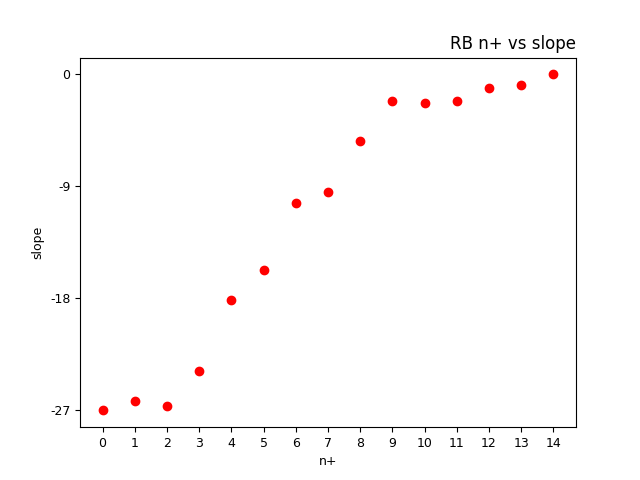
WR:
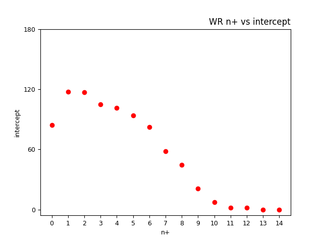
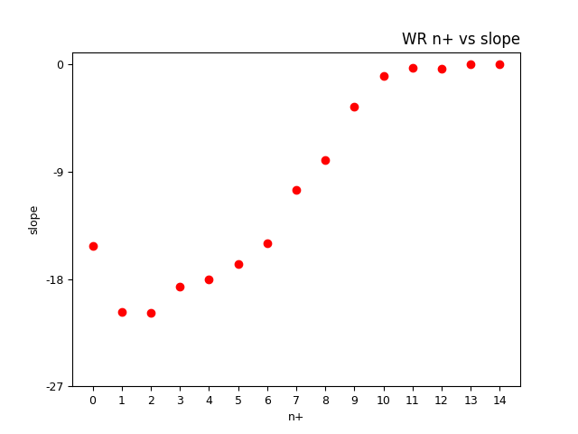
TE:
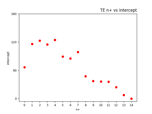
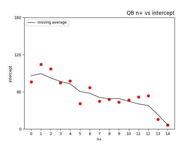
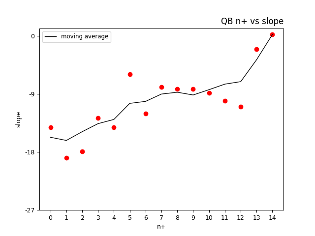
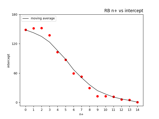
Similar to how these parameters needed to be adjusted for the fvpg predictor variable, the same goes for the variable ln(draft_capital). Slopes, and intercepts adhere to a general trend, and as such should follow a smooth transition instead of bouncing around. On one hand it's a bit easier for ln(draft_capital) because there's only one controlling variable, n+; on the other, there's no simple way to apply a function to the trend. As such, a variation of the to smooth the parameters. The black line in the following images represents the adjusted values.
QB:
RB:
WR:
TE: