smoothing
The purpose of is to remove from data in favor of an overall trend.
Reviewing slopes from regression iterations already completed, notice variance from one age to the next, masking a pattern.
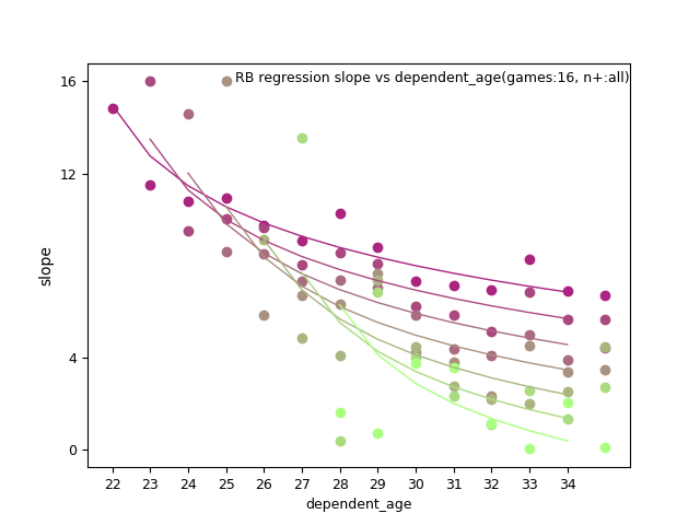
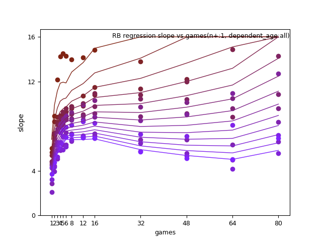
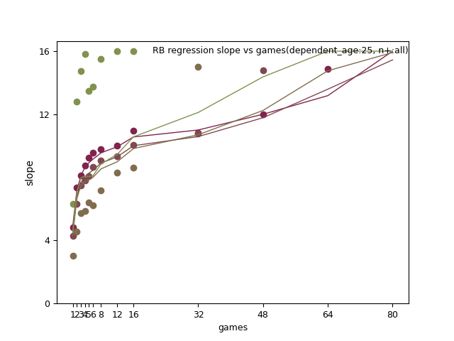
Shown below are slope parameters vs dependent_age(d_age) for RB:
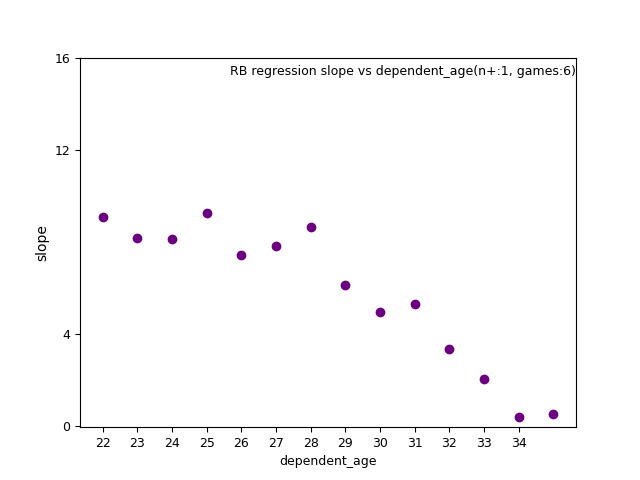
Smoothing is clearly necessary here because prediction should not change randomly from one age to the next.
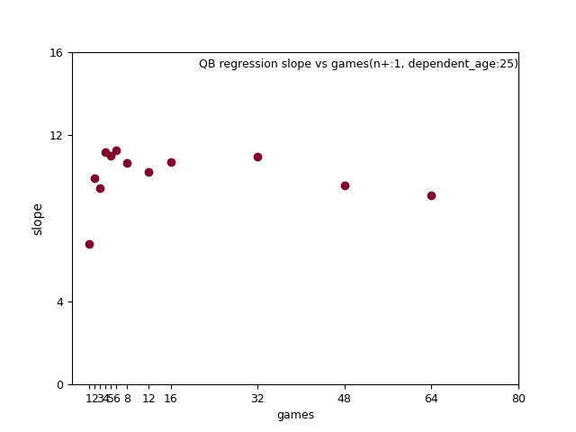
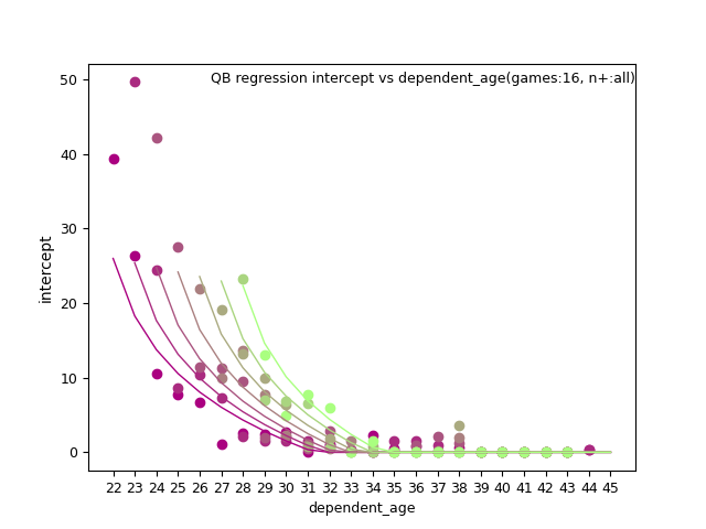
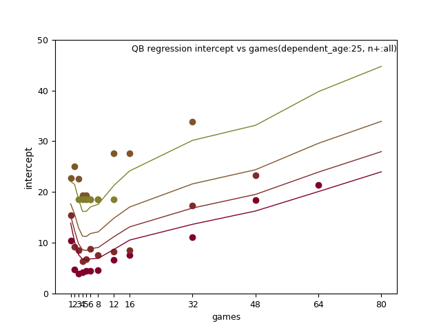
For example, consider the image below for QB:
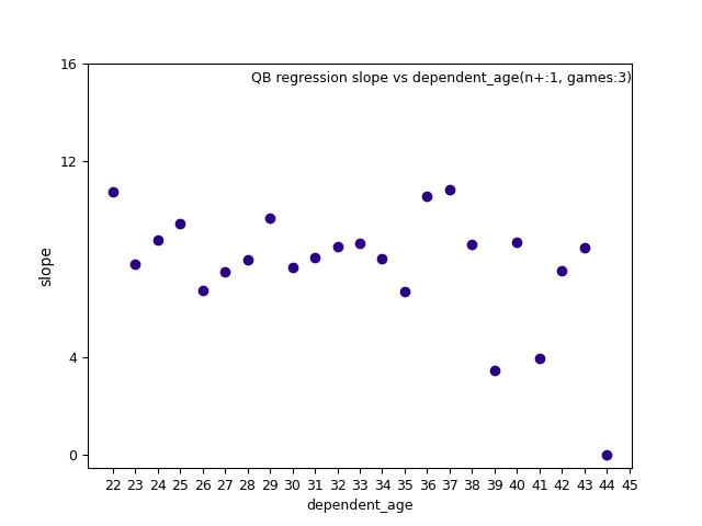
It doesn't make sense for fantasy_value_per_game(fvpg) age 29 to predict better than age 26, but worse than age 37.
A consistency needs to be established.
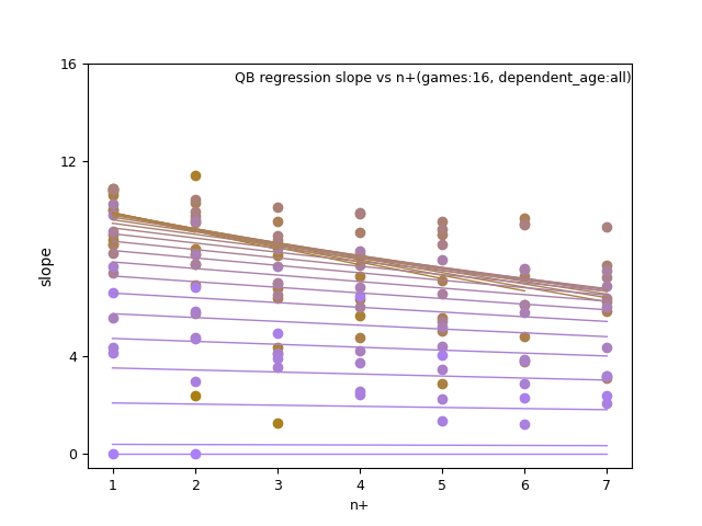
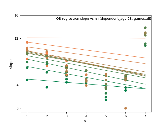
The variables which are found to show a trend are age, career games, and time lag as well. Another variable needs to be defined to represent the time lag, n_plus(n+) equals dependent_age minus predictive_age(p_age). You can think of this as years into the future, higher values represent a longer time span.
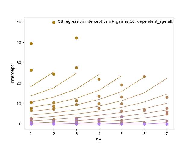
Slope and intercept show with n+, d_age, games_played, and p_age. The introduction of the n+ variable means only one of d_age and p_age is needed.
Tho associations are clear, trends are not straight forward;
as in they are not linear in all cases.
To complicate matters, the trends differ by , and for slope/intercept.
Specificially the age variable was strange.
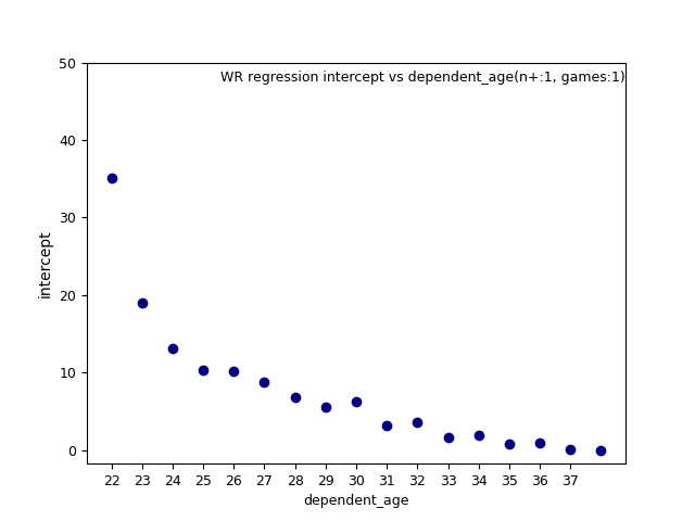
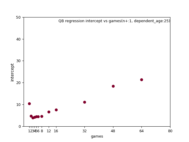
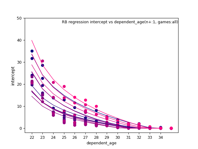
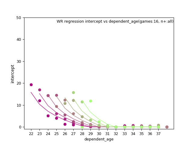
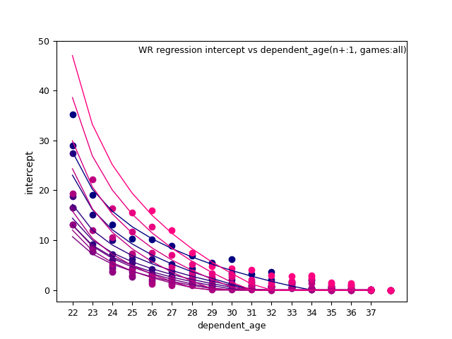
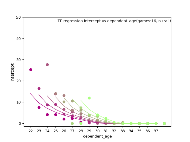
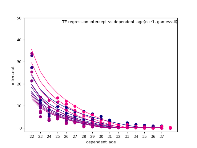
Here's an example of intercept vs d_age, appearing to have sort of a logarthmic trend:
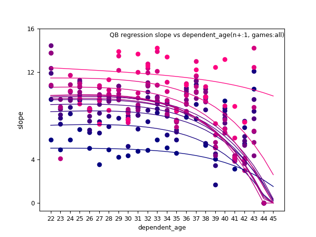
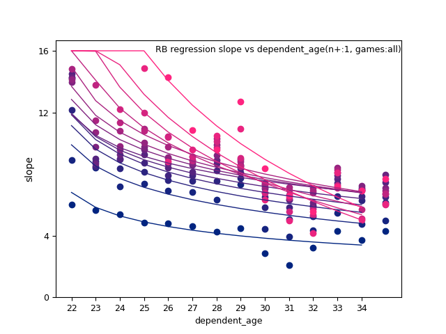
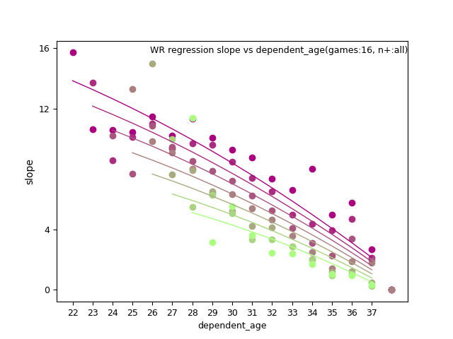
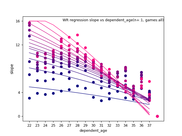
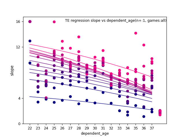
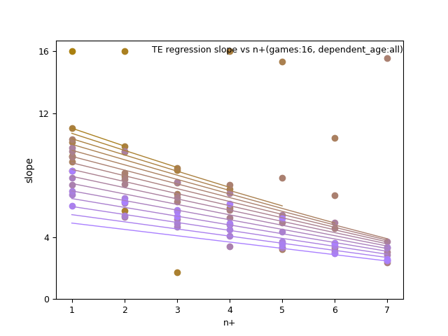
And then the opposite for slope vs d_age:
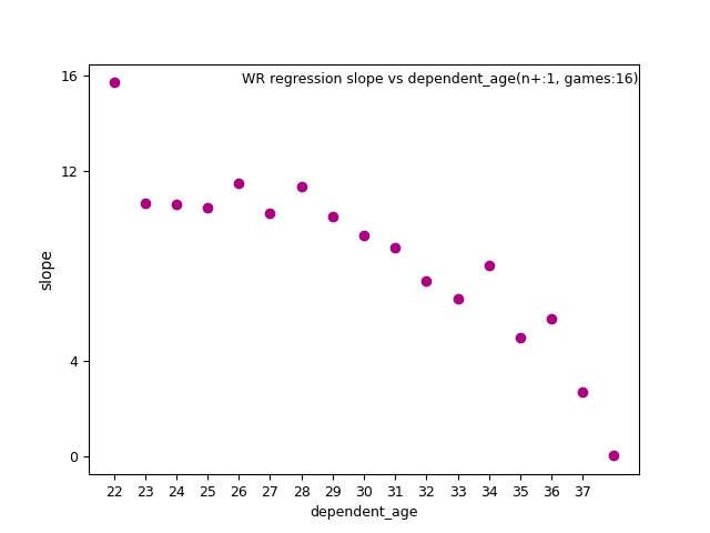
To address these discrepancies more are needed.
Here's the ones which were used: d_age, d_age2, d_age8, and ln(p_age-21).
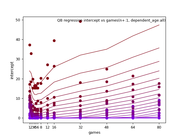
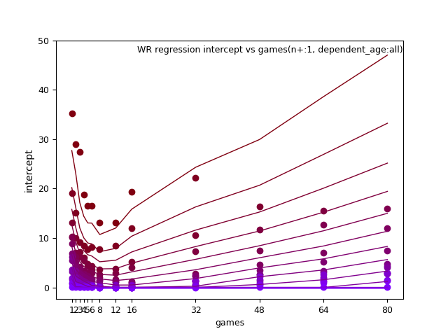
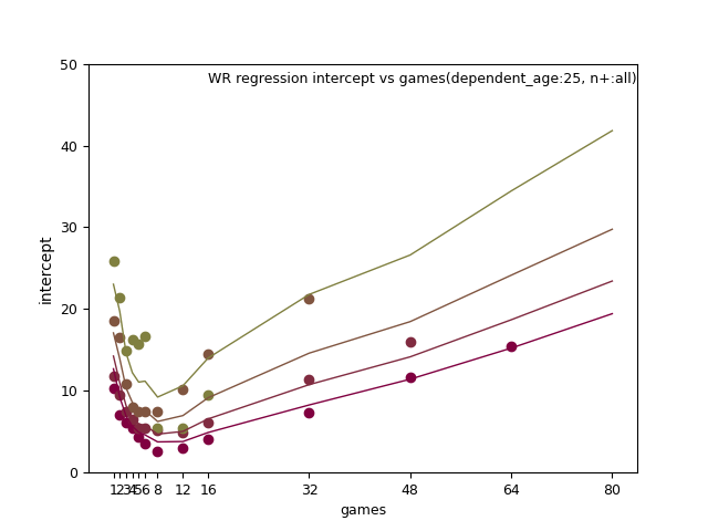
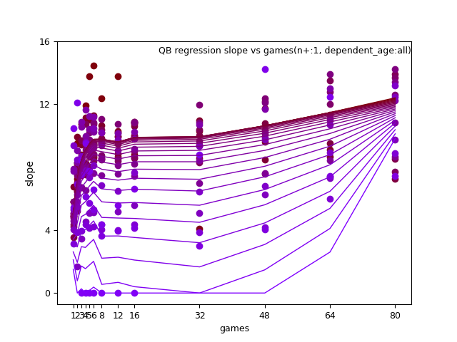
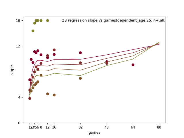
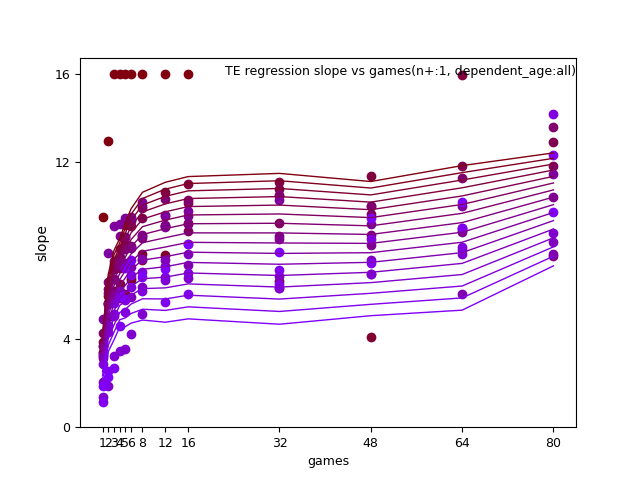
I found games_played(gp) was even more complicated.
It seems to follow a line of best fit, but this function didn't work out in real life.
For one thing, there's a noticable hitch, happening to correspond with the in the intercept.
I could make no sense of this interaction, so as a work around the smoothing portion cycles gp in lieu of capturing the trend mathmatically.
This process is similar to the model's regression iterations.
Fortunately, smoothing by variables n+ and d_age also blends somewhat on the gp variable.
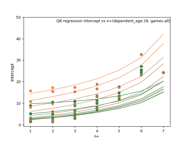
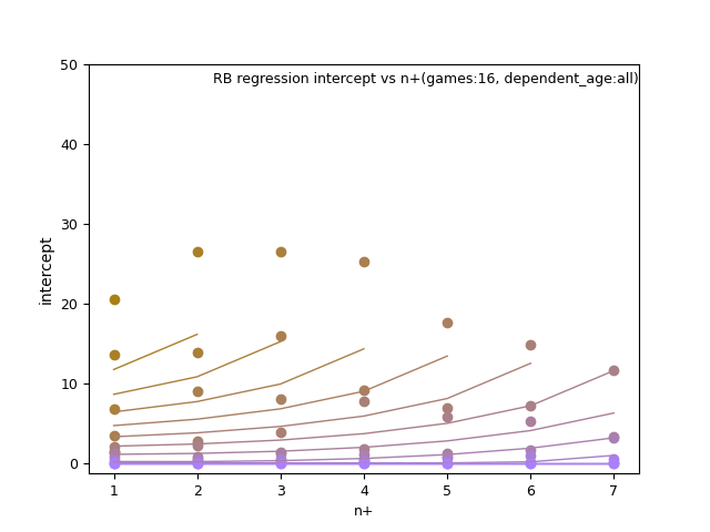
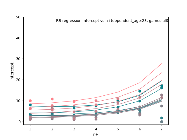
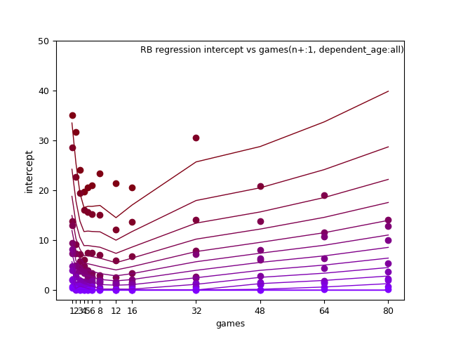
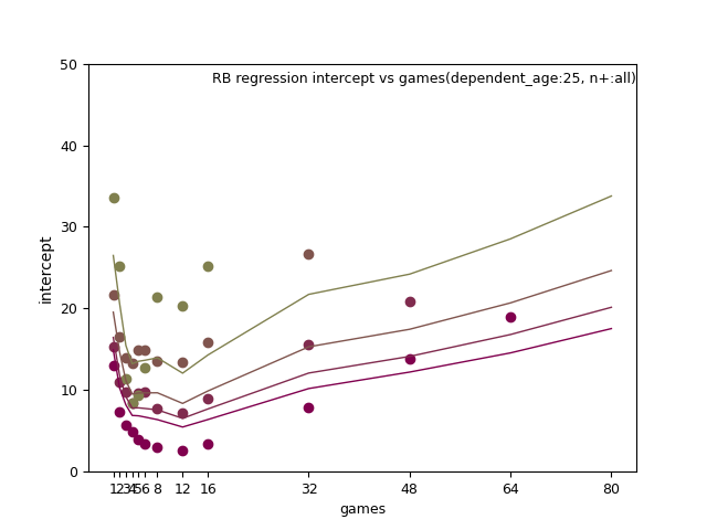
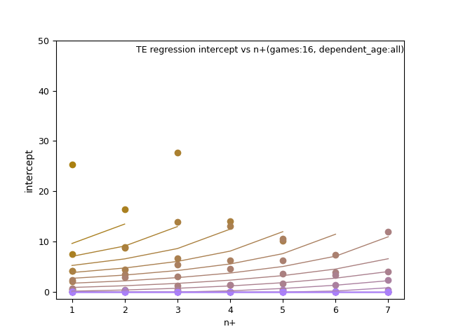
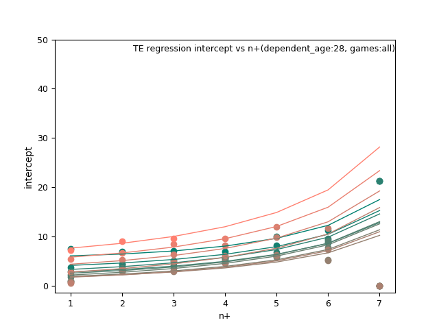
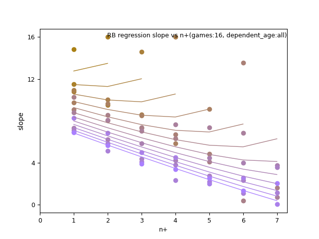
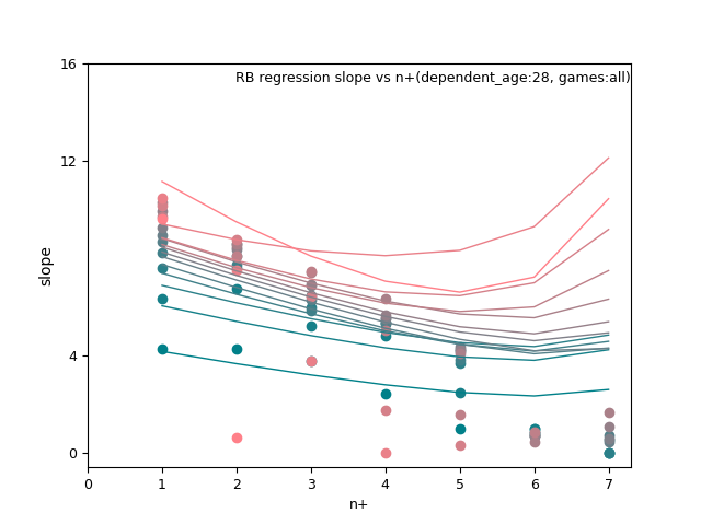
I noticed between d_age and n+, the best fit parameters may change along the lines of d_age when n+ changes. This indicates a potential ; meaning these two variables may work together so to speak. An interaction variable was defined to be included in the regression as n+ * d_age.
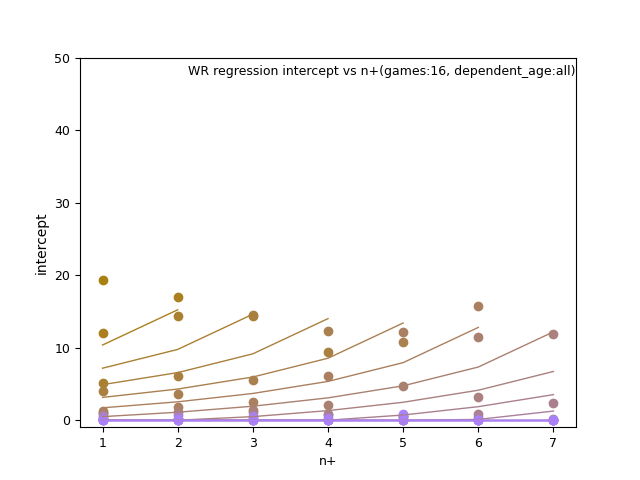
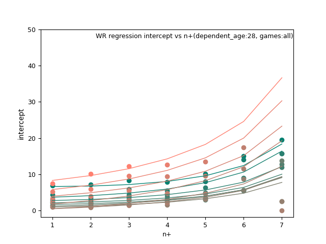
There are a lot of images to view here, where you can change axis, games_played and trends of best fit.
The smoothing operation, again cycles thru the same ranges of gp as in the model's regression portion: 1-1, 2-2, 3-3, 4-4, 5-5, 6-6, 7-8, 9-12, 13-16, 17-32, 33-48, 49-64, 65-80. Except for the ln(draft) and draft_capital, wherein gp equals 0. This time taking advantange of ; WLS is pretty much the same as , but adds a confidence factor to each data point.
The weight value represents a level of confidence associated with each regression, which the smoothing function should account.
for example, is a general measure of fit, changes with dependent_age:
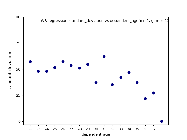
Also appears related to the number of observations as well:
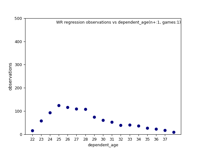
Here are images of standard deviation for each iteration and observations. I decided to use observations for the weighted values because of their uniformity. In fact, obervations show the least variance of all the regression parameters. You can judge for yourself for slope and intercept. There's a lot of images there to view, where you can change the axis, and view different trends of best fit.
Notice a combination of variables fits the data better than just one. Therefore, instead of with a single independent variable, is needed. Some form of d_age, n+, and their joint interaction had an impact on the slope and intercept terms; tho these combinations differed by predictor variable and slope or inercept.
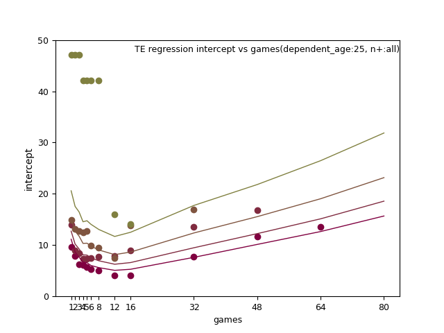
Intercept used ln(p_age-20) and n+.
But trends of best fit changed by position for slope.
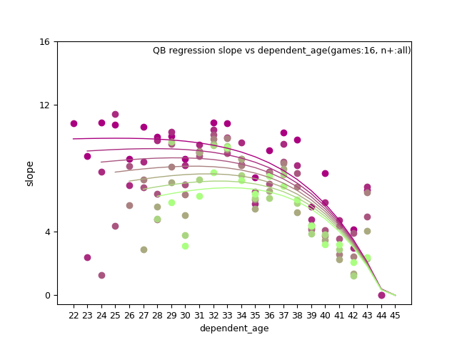
QB: d_age8, n+, and n+ x d_age
RB: ln(p_age-20), n+, and n+ x d_age
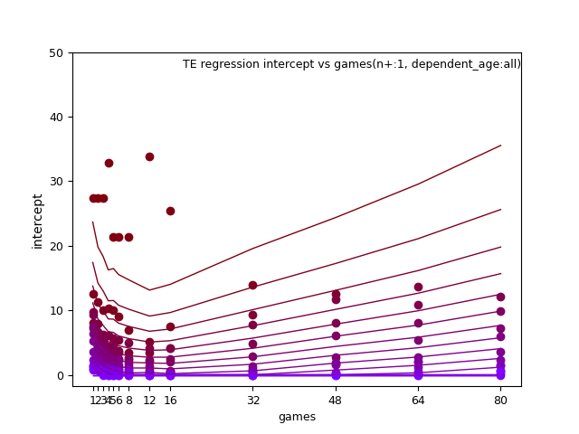
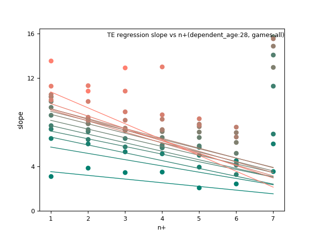
WR/TE: d_age2, n+, and n+ x d_age
fantasy_value_per_game, intercept:
QB:

RB:
WR:
TE:
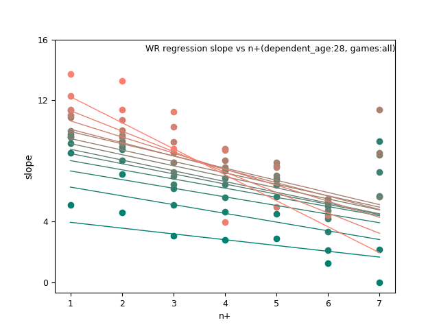
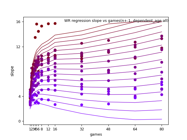
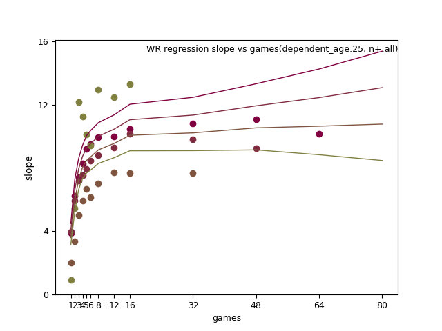
fantasy_value_per_game, slope:
QB:
RB:
WR:

TE:


Again here are all the graphs for slope and intercept so you can check my work regarding the best combination of regression variables.